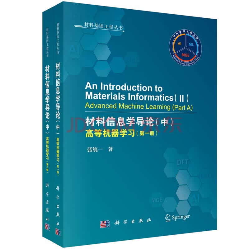
《An Introduction to Materials Informatics（II）Advanced Machine Learning（Part A）（材料信息学导论（中）高等机器学习）（一、二册）》稿是材料信息学系列简介的第二《An Introduction to Materials Informatics（II）Advanced Machine Learning（Part A）（材料信息学导论（中）高等机器学习）（一、二册）》。系列**《An Introduction to Materials Informatics（II）Advanced Machine Learning（Part A）（材料信息学导论（中）高等机器学习）（一、二册）》名为《材料信息学导论(I)：机器学习基础》，专讲**机器学习或者统计学习。如在**《An Introduction to Materials Informatics（II）Advanced Machine Learning（Part A）（材料信息学导论（中）高等机器学习）（一、二册）》第1章中所述，自适应和迭代式的主动学习是数据驱动材料逆向设计的好方法。当考虑实验不确定性和AI模型不确定性时，全局贝叶斯优化和基于群体的优化在材料信息学和主动学习中被广泛地用于平衡探索和利用。《An Introduction to Materials Informatics（II）Advanced Machine Learning（Part A）（材料信息学导论（中）高等机器学习）（一、二册）》第1章和第2章分别描述了**的全局贝叶斯优化和群体优化算法，并讲解了帕累托前沿。第3章迁移学习和多任务学习通过整合多个源域的数据能够提高AI模型的鲁棒性。迁移学习和多任务学习中即使用了许多**机器学习算法，也使用了大量深度学习算法。《An Introduction to Materials Informatics（II）Advanced Machine Learning（Part A）（材料信息学导论（中）高等机器学习）（一、二册）》的第4-9章都是关于深度学习的，包括第4章的卷积神经网络（CNNs）、第5章的递归神经网络（RNNs）和长短期记忆网络（LSTMs）、第6章的图神经网络（GNN）、第7章的生成对抗网络（GANs）、第8章的扩散模型、第9章的Transformers以及第10章的物理信息神经网络（PINN）。除了监督学习和无监督学习，强化学习（RL）被视为第三种机器学习范式，因此第11章介绍了强化学习和深度强化学习。

Contents
Part A Optimization and Learning Strategies
1 Bayesian Global Optimization 3
1.1 Gaussian Process Regression (GPR)， Ordinary Kriging (OK)， and Jones Approach 6
1.2 Acquisition Functions 31
1.2.1 Expected Improvement (EI) 31
1.2.2 Expected Improvement with Plugin (EI Plugin) 44
1.2.3 The Reinterpolation Procedure 47
1.2.4 Augmented Expected Improvement (AEI) 51
1.2.5 Upper Confidence Bound (UCB) and Minimum Quantile (MQ) 59
1.2.6 Probability of Improvement (PI or PoI) 66
1.2.7 Expected Quantile Improvement (EQI) 73
1.2.8 Knowledge Gradient (KG) 83
1.2.9 Entropy Search (ES) 94
1.2.10 Utility Functions and Acquisition Functions for Classification 99
1.3 Multiobjective Optimization 108
1.3.1 Classical Methods for Multiobjective Optimization 110
1.3.2 Nondominated Feature Points (Solutions) and Pareto Front (Srinivas and Deb 1791–1994) 114
1.3.3 Hypervolume Improvement 128
References 150
2 Swarm-Based Optimization Algorithms 155
2.1 Particle Swarm Optimization (PSO) 155
2.2 Whale Optimization Algorithm (WOA) 165
2.2.1 Shrinking Encircling Method 167
2.2.2 Bubble-Net Method 168
2.2.3 Exploration in WOA: Search for the Prey 169
2.3 Ant Colony Optimization (ACO) 177
References 184
3 Transfer Learning 187
3.1 Basic Concepts 188
3.1.1 Definitions 188
3.1.2 Categorization of Transfer Learning 189
3.2 AdaBoost Transfer Learning 190
3.2.1 AdaBoost Transfer Classification 190
3.2.2 AdaBoost Transfer Regression 208
3.3 Instance-Transfer Learning 235
3.3.1 Kernel Mean Matching (KMM) Method in Linear Regression 238
3.3.2 KMM in Support Vector Machine 239
3.4 Mapping Transfer Learning and Neural Network-Based Transfer Learning 245
3.4.1 Deep Adaptation Network (DAN) 252
3.4.2 Domain-Adversarial Neural Network (DANN) 271
3.4.3 Wasserstein Distance-Based Deep Transfer Learning (WD-DTL) 278
3.5 Feature Augmentation 289
References 296
4 Reinforcement Learning 299
4.1 The K-armed Bandit Algorithm 300
4.1.1 The Softmax Method 302
4.1.2 The Normal Distribution Awards 310
4.1.3 The Upper Bound Method 311
4.1.4 The Incremental Method with a Constant Step-Size 315
4.2 The Gradient Bandit Algorithm 317
4.3 Markov Decision Process (MDP) 320
4.4 Dynamic Programming 348
4.4.1 Policy Iteration—Policy Evaluation 349
4.4.2 Policy Iteration—Policy Improvement 351
4.4.3 Value Iteration 354
4.4.4 Variants of Dynamic Programming 358
4.5 Monte Carlo Methods 365
4.5.1 Monte Carlo Policy Evaluation 365
4.5.2 Monte Carlo Policy Estimation 370
4.5.3 Monte Carlo Policy Improvement 373
4.5.4 On-Policy Monte Carlo Control 376
4.5.5 Off-Policy Monte Carlo Estimation 379
4.5.6 Off-Policy Monte Carlo Control 388
4.6 Temporal-Difference (TD) Learning 393
4.6.1 TD Prediction 393
4.6.2 Q-Learning and Expected Sarsa 397
4.6.3 Double Q-Learning 401
4.6.4 Neural Fitted Q Iteration (NFQ) 403
4.7 Deep Reinforcement Learning 410
4.7.1 Deep Q-Networks (DQNs) 410
4.7.2 Policy Gradient Algorithms 424
4.7.3 Deep Deterministic Policy Gradient (DDPG) Algorithm 432
References 440
Part B Advanced Neural Networks
5 Convolutional Neural Networks 445
5.1 Convolution and Cross-Correlation of Two Functions 445
5.2 The Architecture of CNNs 447
5.3 How CNN Works 451
5.4 Finite Element Analysis Network (FEA-Net) 473
References 486
6 Recurrent， Long Short-Term Memory， and Gated Recurrent Unit Neural Networks 489
6.1 Recurrent Neural Network (RNN) 489
6.1.1 Backpropagation Through Time (BPTT) 494
6.1.2 Gradient Vanishing and Exploding in RNNs 505
6.2 Long Short-Term Memory (LSTM) 507
6.2.1 BPTT in LSTM 513
6.3 Gated Recurrent Unit (GRU) 518
6.4 Applications of LSTMs in Materials Informatics 524
References 534
7 Graph Neural Networks (GNNs) 535
7.1 Graph Representation 536
7.1.1 Definitions of Graph 538
7.2 Recurrent GNNs (RecGNNs) 542
7.2.1 Convergence-Based Recurrent GNNs 542
7.2.2 Gate-Based Recurrent GNNs 550
7.3 Convolutional Graph Neural Networks 594
7.3.1 Spectral-Based ConvGNNs 594
7.3.2 ChebNet 611
7.3.3 Graph Convolutional Network (GCN) 615
7.3.4 Spatial-Based ConvGNNs 618
7.3.5 Diffusion Convolutional Neural Networks (DCNN) 621
7.3.6 Deep Graph Convolutional Neural Network (DGCNN) 627
7.3.7 Parametric Graph Convolution (PGC)-DGCNN 631
7.3.8 Message Passing Neural Networks (MPNNs) 636
7.3.9 Graph Isomorphism Network (GIN) 640
7.3.10 GraphSAGE (Sample and Aggregation) 642
7.3.11 Crystal Graph Convolutional Neural Networks (CGCNN) 647
7.4 Variational Graph Auto-Encoders (VGAE) 654
7.5 Attention-Based GNNs 658
7.5.1 Graph Attention Networks (GATs) 658
7.5.2 Crystal Edge Graph Attention Neural Network (CEGANN) 662
7.5.3 Matformer 671
7.6 Temporal Graph Convolutional Network (T-GCN) 683
7.7 Fingerprints of Molecules in CEGANN 686
R

Part A Optimization and Learning Strategies
　　Chapter 1 Bayesian Global Optimization
　　As described in Chap. 1 of An Introduction to Materials Informatics (I): The Elements of Machine Learning， materials informatics employs adaptive active learning， in which one material property (or multiple material properties) is called the output， target， objective， or response and the input feature variables are material composition， processing， testing conditions， or/and service environments， etc. Microstructures of a material could be features， responses， or hidden state variables， depending on the problems under study. For a material with a given chemical composition， different material processing methods and conditions render various microstructures to the material， which in turn determine the macroscopic properties and the performance of the material. Adaptive active learning is a dynamic iterative process and initially starts from experiment or/and computation to generate a certain amount of data. Figure 1.1 shows schematically the iteration loop of Bayesian global optimization. Material scientists and engineers design and conduct experiments or/and computations based on investigation tasks and domain knowledge， with the goal of developing excellent material properties and discovering the relationships among macroscopic properties， chemical composition， processing conditions， or/and service environments. In the machine learning (ML) field， design of experiments (DOE) suggests experimental feature points， at which the expected experimental results yield material properties that are as excellent as possible， and/or provide as much information as possible about the input–output relationship. In materials design via computation， computation might be regarded as a generalized form of experiments. The observed data at the DOE points naturally form an initial dataset. A surrogate model， a ML model or an analytical theoretical model， is developed with the current dataset to find a relationship between the input and output variables. Bayesian global optimization is a probabilistic and recursive method that accounts for uncertainties in both experiment and model prediction， meaning that the model prediction should contain the expectation and variance of an objective. An acquisition function， as the core of Bayesian global optimization， is used to recommend how to conduct the next experiment or/and computation by balancing exploration and exploitation. Exploration means to gain more information from un-investigated region of feature space， while exploitation takes the profit of information already obtained. The recommended experiment or/and computation is conducted and the new results of experiment or/and computation validate the ML prediction and simultaneously are fed back to the dataset for the following cycle of iterations in the adaptive active learning loop. The iteration goes on until reaching the designed objective， while adaptive and active learning， in principle， never ends and the accumulated data are always valuable. The basic and essential ML methods and algorithms are introduced in An Introduction to Materials Informatics (I): The Elements of Machine Learning. This chapter presents how to make a recommendation to the next step of experiment or/and computation， when there are uncertainties (noises) in data and in prediction. Figure 1.1 highlights the recommendation， called the new design of experiment or/and computation in materials informatics and termed the feature infill or acquisition in AI and ML， based on Bayesian global optimization with uncertainties (noises). There are various infill criteria and acquisition functions with common characteristics and individual distinctions. As emphasized always， the knowledge of materials science and engineering is the hub of active learning in materials informatics， because without the domain knowledge it will be hard to understand and analyze materials data. High-level domain knowledge guides each step in the active learning process and reduces the gap between information and knowledge. A trustful development of novel promising materials and great scientific advancement depends on the knowledge retrieval， acquisition， representation， management， knowledge level modeling， etc.， in the active learning， where the new design of experiment or/and computation plays a crucial role. The exploration exploitation tradeoff is also the hub in Bayesian global optimization， as illustrated in Fig. 1.1.
　　Fig. 1.1 Schematic of dynamic active learning. Domain knowledge is the hub in the adaptive iteration process， while exploration exploitation tradeoff is the hub in Bayesian global optimization
　　To consider uncertainties in data and in predictions， the probabilistic approach believes that an observed response is randomly drawing a sample such that
　　where yi(j)， μi(mi)， and εi(j) (i = 1， ，n) denote the response value， the expectation (mean) and error of feature point